Understanding Elasto-Plastic Material Models in ANSYS Mechanical

Introduction

In the world of structural simulations, material behavior plays a crucial role in predicting how materials respond under different loading conditions. Material models are mathematical descriptions of how materials behave under loads. They define how stress and strain are related. Depending on the material and the expected loading, different models like linear elastic, plastic, hyperelastic, or viscoelastic are used.

Materials typically exhibit elastic behavior at low stress levels, returning to their original shape upon unloading. However, beyond a certain stress threshold, known as the yield point, materials undergo plastic deformation, resulting in permanent changes to their shape. To accurately capture this transition from reversible to irreversible behavior, elasto-plastic material models are used, resulting in more realistic and reliable simulation outcomes.

Elasto-plastic models describe materials that initially respond elastically — following Hooke's Law — and then transition into plasticity once the yield point is exceeded. By modeling both elastic and plastic behaviors together, these models are crucial for predicting material failure, optimizing component designs, and enhancing material performance under extreme loading conditions.

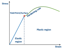
Key Features of Elasto-Plasticity (refer Figure 1)

1. Elastic Region – The material follows Hooke's Law (stress is proportional to strain).
2. Yield Point / Surface – The limit beyond which permanent deformation begins. In 1-D loading, it's a single yield point; in 3-D loading, it extends into a yield surface.
3. Plastic Region – Irreversible deformation occurs.
4. Hardening Rule – Describes how the material resists further plastic deformation.

In plasticity theory, materials exhibit different behaviors depending on whether their plastic response is influenced by strain rate, which is affected by the rate of loading. This leads to two main categories: rate-independent plasticity, where the material's plastic behavior remains unchanged regardless of loading speed, and rate-dependent plasticity, where yield stress increases with faster loading due to strain rate effects.

This strain rate effect refers to how a material's response changes with deformation speed, making materials stronger as strain rate increases. It is particularly important in applications involving dynamic or high-speed loading, such as impact, crash, explosion, and metal forming processes. The present discussion would be limited to rate independent material models.

The constitutive models for elastic-plastic behavior start with a decomposition of the total strain into elastic and plastic parts. The stress is proportional to the elastic strain, and the evolution of plastic strain is a result of the plasticity model.

1. Elastic Strain – Temporary deformation, where the material returns to its original shape.
2. Plastic Strain – Permanent deformation, where the material does not return to its original shape.

There are 3 essential characteristics of the plastic constitutive models,

1. Yield Criterion – Defines when a material transitions from elastic to plastic behavior. i.e., defines the point where the material stops behaving elastically and starts deforming plastically.
2. Flow Rule – Determines how much plastic strain develops when the material is loaded beyond its yield point. It determines the increment in plastic strain from the increment in load in terms of the plastic multiplier and the plastic potential.
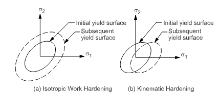
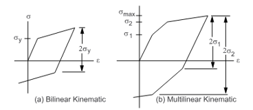
3. Hardening Rule – Describes how the yield criterion evolves during plastic deformation. As loading continues, stress and plastic strain increase, strengthening the material. The two common types are isotropic and kinematic hardening (refer Figure 2).

Types of Hardening

• Isotropic Hardening – The yield surface expands uniformly, meaning the material hardens equally in all directions. It is suitable for modeling the behavior of materials under monotonic loading and elastic unloading but often does not give good results for structures that experience plastic deformation after a load reversal from a plastic state.
• Kinematic Hardening – The yield surface translates (shifts) in stress space, allowing the material to simulate cyclic loading effects, such as repeated bending. It is commonly used to model phenomena like the Bauschinger effect, where the compressive yield strength decreases following tensile yielding.

Types of Elasto-Plastic Material Models in ANSYS Mechanical

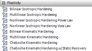
Ansys Mechanical provides a comprehensive set of elasto-plastic constitutive models (simply Plasticity models), enabling engineers to accurately simulate material response in industries like automotive, aerospace, manufacturing, and civil engineering.

The figure above shows the hardening models available in Ansys Mechanical, including both isotropic and kinematic hardening options.

1. Isotropic Hardening Models

These models assume that the yield surface expands uniformly in all directions as the material hardens. They are suitable for monotonic loading conditions.

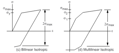
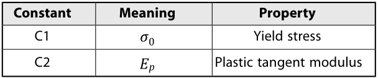
a) Bilinear Isotropic Hardening – Uses a constant plastic modulus after yielding. The following table lists the required constants:

b) Multilinear Isotropic Hardening – Defines multiple yield points for better accuracy. The behavior of multilinear isotropic hardening is similar to bilinear isotropic hardening except that a multilinear stress versus total or plastic strain curve is used instead of a bilinear curve.

The multilinear hardening behavior is described by a piece-wise linear stress-total strain curve, starting at the origin and defined by sets of positive stress and strain values, as shown in this figure:

c) Nonlinear Isotropic Hardening (Power Law, Voce Law) – Captures more complex hardening behavior using empirical laws.

Power Law Hardening follows a power-law relationship between stress and plastic strain. The following table lists the required constants:

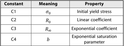
Voce Law Hardening models material behavior where there is rapid initial hardening after yielding, followed by a gradual saturation to a constant stress level. The following table lists the required constants:

2. Kinematic Hardening Models (Accounts for Bauschinger Effect, Cyclic Loading)

Kinematic hardening models shift the yield surface in stress space, making them ideal for cyclic loading applications (e.g., fatigue analysis).

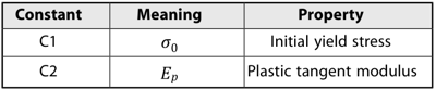
a) Bilinear Kinematic Hardening – A simple model considering cyclic loading effects. It is defined using two constants mentioned below.

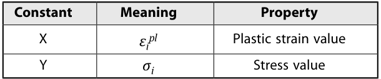
b) Multilinear Kinematic Hardening – Uses multiple stress-strain points for better accuracy. The following table provides details about the constants used in this model, representing the stress and strain values at point i.

c) Nonlinear Kinematic Hardening:

Chaboche Kinematic Hardening – A nonlinear model for cyclic plasticity and progressive plastic deformation under cyclic loading.

Chaboche Kinematic Hardening w/ Static Recovery: Static recovery (also known as thermal recovery) is a feature in kinematic hardening where the backstress (the shift of the yield surface) relaxes over time even when the material is unloaded or under small loads. It represents dislocation rearrangement and reduction of internal stresses during rest periods.

Static recovery is essential for modeling long-term cyclic loading, low-cycle fatigue, and creep-fatigue interactions.

Choosing the Right Elasto-Plastic Model in ANSYS

Conclusion

Elasto-plastic material models in ANSYS Mechanical provide powerful tools to simulate real-world material behavior accurately. Choosing the right model depends on loading conditions, strain rate sensitivity, and material properties. Whether you're analyzing metal forming, impact resistance, or fatigue, using the correct model ensures reliable simulation results.